Workflow Outline

This workflow demonstrates how to discover, filter, and download Harmonized Landsat Sentinel-2 (HLS) imagery using NASA Earthdata Search. Once downloaded, users will use ArcGIS Pro to combine the individual spectral bands into a multi-band composite, configure the symbology for proper visualization, apply an NDVI raster function for basic vegetation analysis, clip the resulting raster to a boundary to focus the area of analysis, and calculate change detection with the raster calculator to quantify and highlight the degree of change.

Data Used

Tools/Tech Used

  • ArcGIS Pro version ≥3.5.2 (requires Esri license)

Find and Download Data via Earthdata Search

  1. Go to Earthdata Search and login.
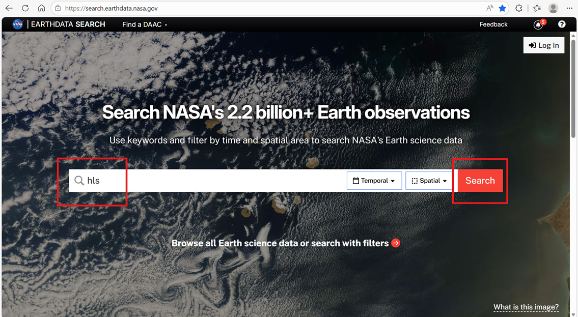
  2. Search for Data.
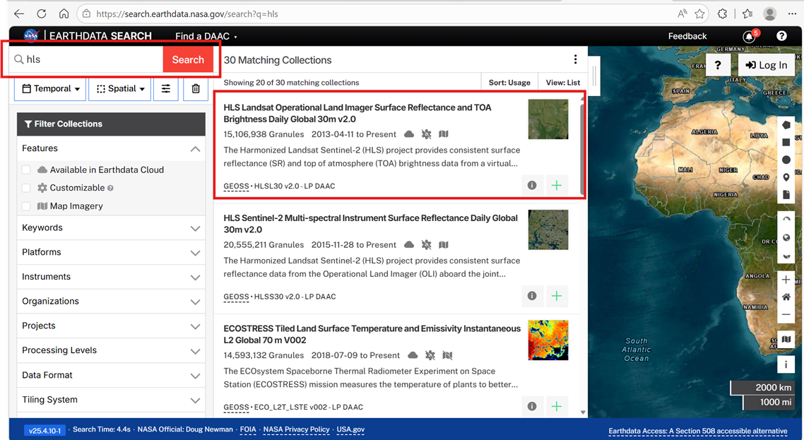
    1. Type in HLS.
    2. Hit Search.
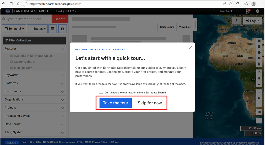
  3. You may receive a pop-up for a guided tour of Earthdata Search. You may either choose to “Take the tour” or “Skip for now.” If this is your first time using Earthdata Search or you want a refresher, we recommend that you take the tour.
Image
Image
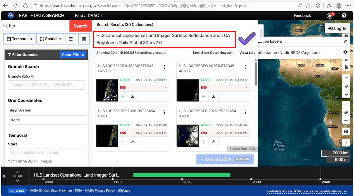
  1. With your search query as “HLS,” look through the matching collections and select “HLS Landsat Operational Land Imager Surface Reflectance and TOA Brightness Daily Global 30m v2.0.” It should be one of the collections at the top of the results.
Image
Image
  1. Filter the data.
    1. Filter spatially.
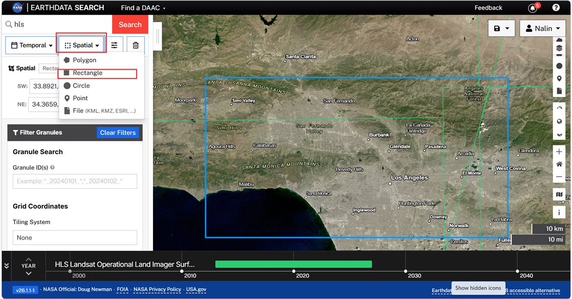
      1. Zoom into an area of interest. In this example, we will be looking at the Santa Monica Mountains outside of Los Angeles, California, in the United States.
      2. Click “Spatial.”
      3. Select “Rectangle.”
      4. Define the area in which you would like to view data granules. See below for the bounding box for this example.
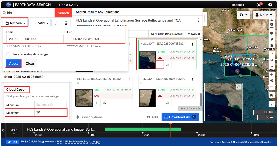
    2. Filter temporally
      1. Enter the start date as “2025-01-01 00:00:00”
      2. Enter the end date as “2025-02-15 23:59:59”
    3. Filter Cloud Cover
      1. Set the max cloud cover as “30”
  2. View and select desired granules to add to your project by pressing the green + sign
    • HLS.L30.T11SLT.2025014T182831
    • HLS.L30.T11SLT.2025006T182824
Image
Image
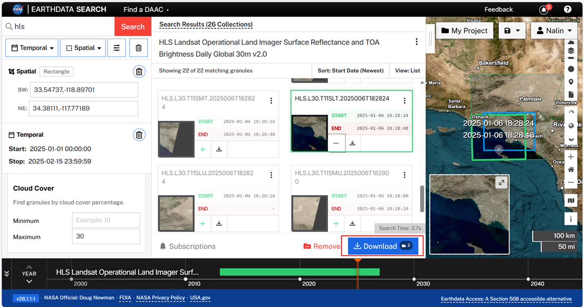
  1. Verify that you have selected your desired data; two granules should be selected.
  2. Hit the blue “Download” button.
Image
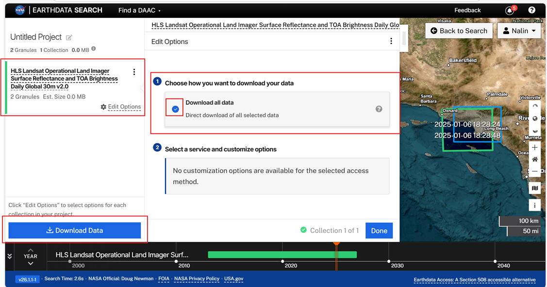
  1. Verify the information is from your desired collection and you have the desired number of granules (two—see below).
  2. Choose the “Download all data” method.
  3. Click the blue “Download Data” button.
Image
  1. Download data.
    1. Once the download status page has finished processing, click “Download Files.”
    2. An “Earthdata Download” message will pop up. Select “Open Earthdata Download” or “Install Earthdata Download as needed.”  If you need to “Install Earthdata Download,” follow the alternative link to download the installer and run it to install the application.
    3. “Earthdata Download” will download the files to the path of your choosing.

Create Multi-Band Composite

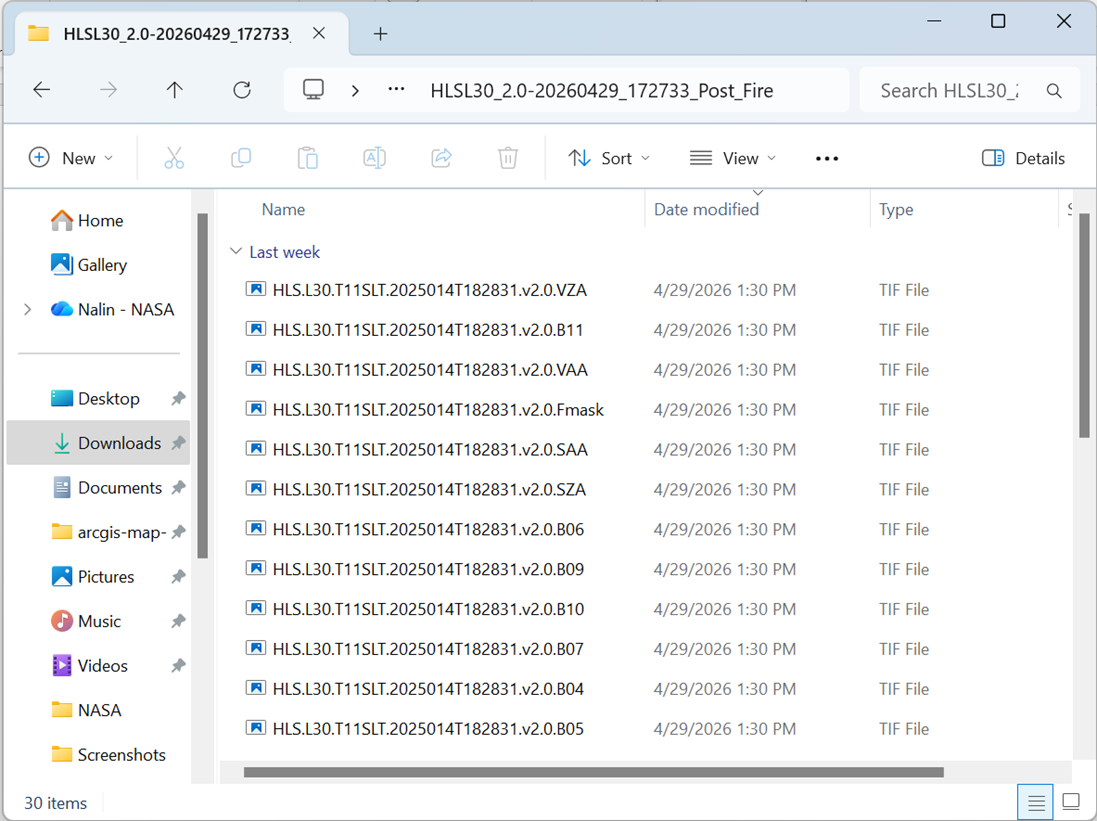
View your downloaded HLS data. Notice how there are many files for each granule. Each file contains one spectral band of the corresponding granule. 

Reference HLS Spectral Bands as needed. We will need to create a multiband composite which will stack and combine these bands into one granule.

Image
  1. Open ArcGIS Pro and create a new project.
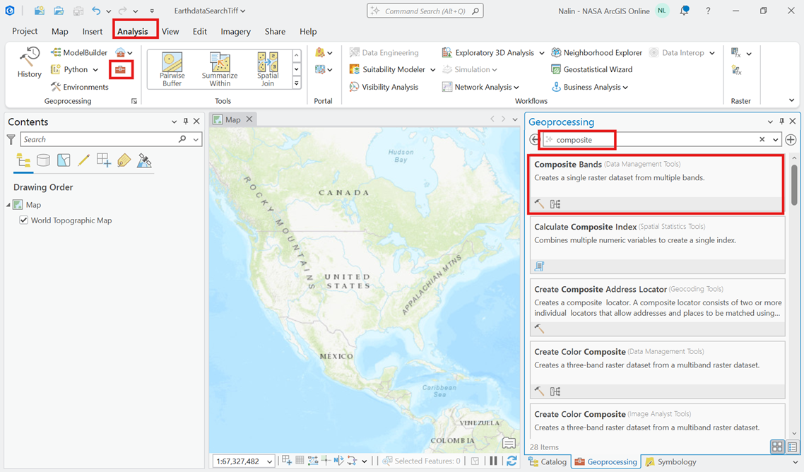
  2. Find the “Composite Bands” tool.
    1. Navigate to the “Analysis” tab.
    2. Click the toolbox icon.
    3. Enter “Composite” into the toolbox search bar.
    4. Select the “Composite Bands” Data Management Tools.
Image
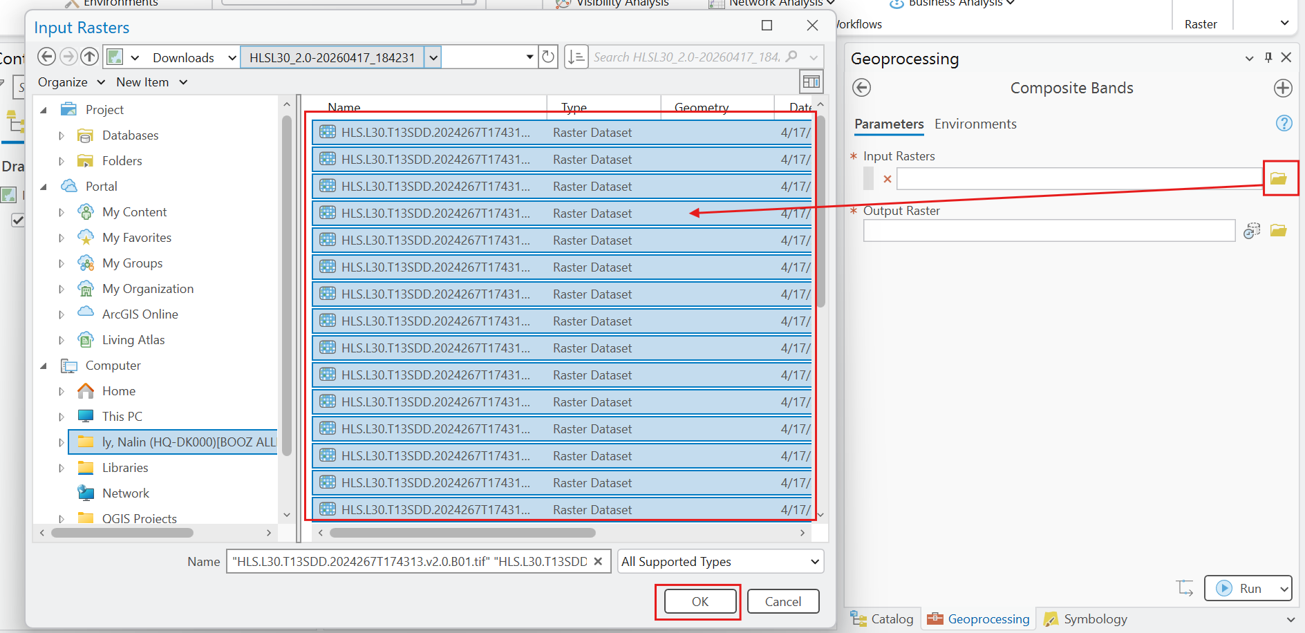
  1. Run the “Composite Bands” Data Management Tool for one of the granules.
    1. Click the folder icon by “Input Rasters.”
    2. Select all files for the corresponding granule (see below).
    3. Hit “OK” to upload them to the tool.
    4. Change the “Output Raster” name by changing ONLY the very end of the path. Remember, you cannot use spaces or “.” in the output name.
    5. Hit “Run.”
  2. Repeat Step 4 to create a multi-band composite for the second granule.
Image

Change Band Combinations

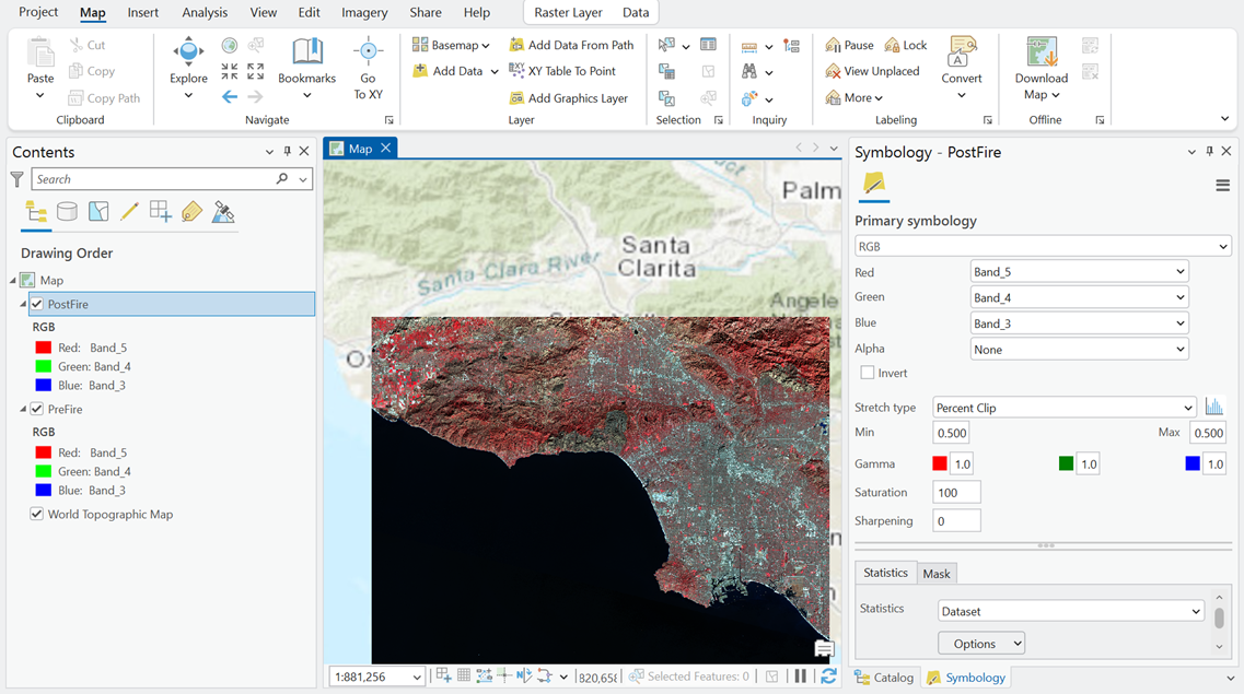
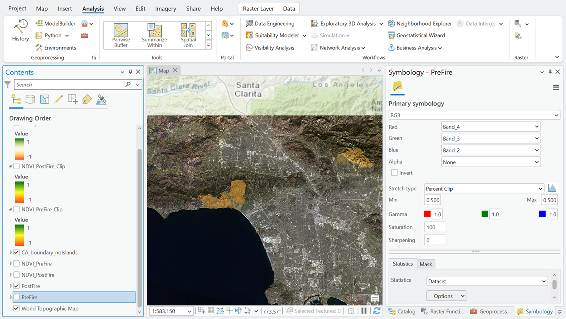
We can manually change band combinations in the symbology to visualize different composites. We can further configure the imagery with other settings such as Stretch type, Gamma, Saturation, etc. For more information, review ArcGIS Imagery Symbology Documentation

  1. Right click on the mosaic dataset and open “Symbology.”
  2. Change band combinations to desired composite. Reference HLS Spectral Bands as needed.
    1. When changing the stretch type, you may be prompted to calculate statistics. Select “Yes.”
    2. In the screenshots provided below, we can see a false-color composite band combination. The stretch type has been set to Percent Clip with min and max clipped at 0.5.
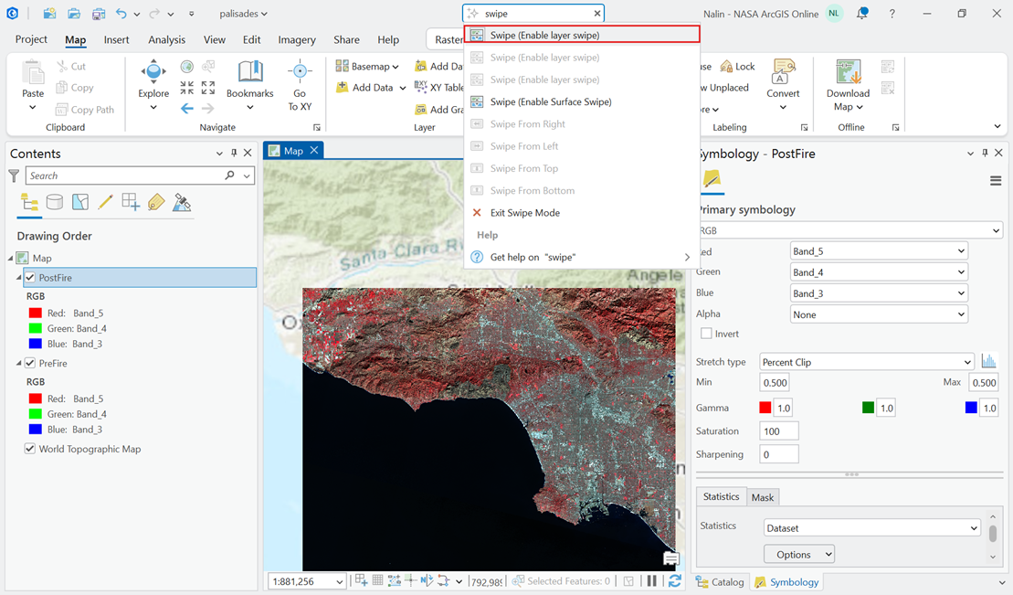
    3. Consider utilizing the “Swipe” tool to compare differences between the two layers.
Image
Image

Apply an NDVI Raster Function

Let's do some basic imagery analysis by applying an NDVI Raster Function. NDVI (Normalized Difference Vegetation Index) is a commonly used index that highlights vegetation by comparing near-infrared and red-light reflectance. 

NDVI helps distinguish healthy vegetation from bare ground, water, and urban areas based on how strongly plants reflect and absorb light. This is useful for fire monitoring, as lower values can indicate vegetation stress, burn scars, or areas impacted by wildfire.

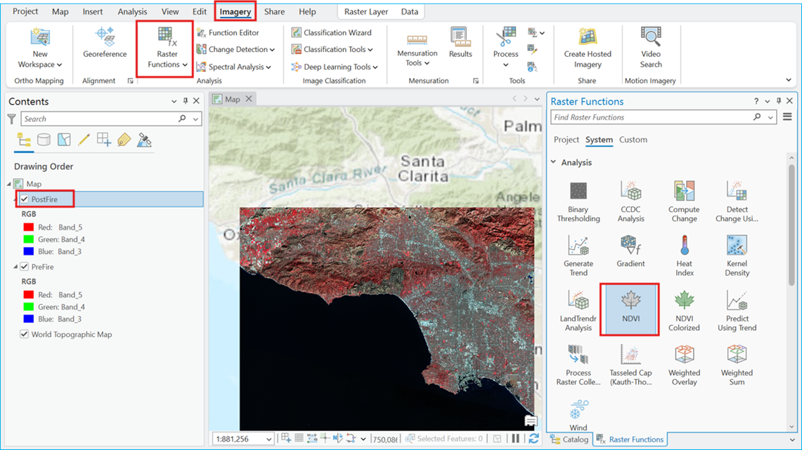
  1. Navigate to the “Imagery” tab and select “Raster Functions.”
  2. Select the “NDVI” icon from the “Raster Functions” pane.
  3. For “Raster,” enter one of the rasters we’re working with.
  4. Enter band “4” for the “Visible Band ID.”
  5. Enter band “5” for the “Infrared Band ID.”
  6. Check the “Scientific Output” box.
  7. Hit “Create new layer."
  8. Repeat for the second raster.
Image

The resulting NDVI may not look properly configured. We will adjust the symbology to properly visualize it.

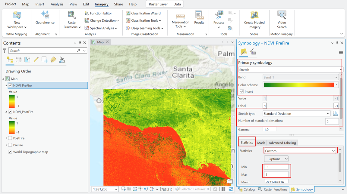
  1. Open the NDVI’s symbology pane.
  2. Set “Statistics” to “Custom” and define “Min” as “-1” and “Max” as “1” to set the proper range.
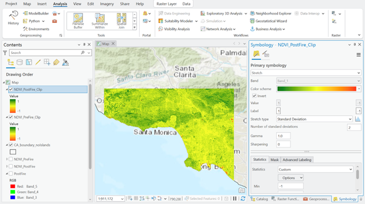
  3. Change the color scheme to a red-yellow-green color ramp. We have checked the “Invert” box for the selected color ramp for red to indicate low values and green to indicate high values
  4. Change the “Stretch type” to “Standard Deviation” and ensure the “Number of standard deviations” is “2.”
  5. Reference ArcGIS Imagery Symbology Documentation to continue to configure the symbology as desired.
Image

Clip Raster to Boundary

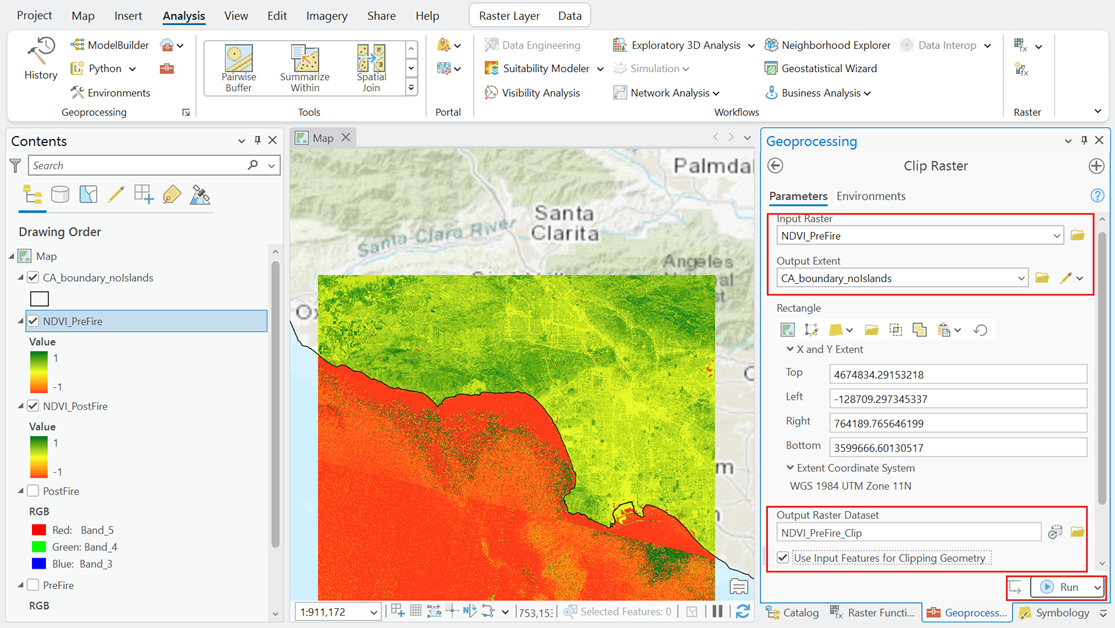
Let’s clip the rasters to the boundary of California to exclude ocean areas from our visualization and analysis. This ensures the results focus only on land-based vegetation conditions relevant to fire monitoring. To do this, we will first add a boundary layer to the map.

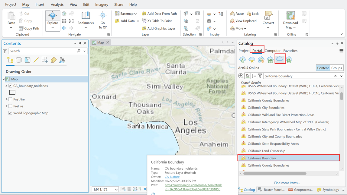
  1. Navigate to the “Portal” tab under the “Catalog” pane.
  2. Under “ArcGIS Online” (Cloud Icon), search for “California Boundary” and add an appropriate boundary layer to the map.
Image
  1. Clip the raster to the boundary.
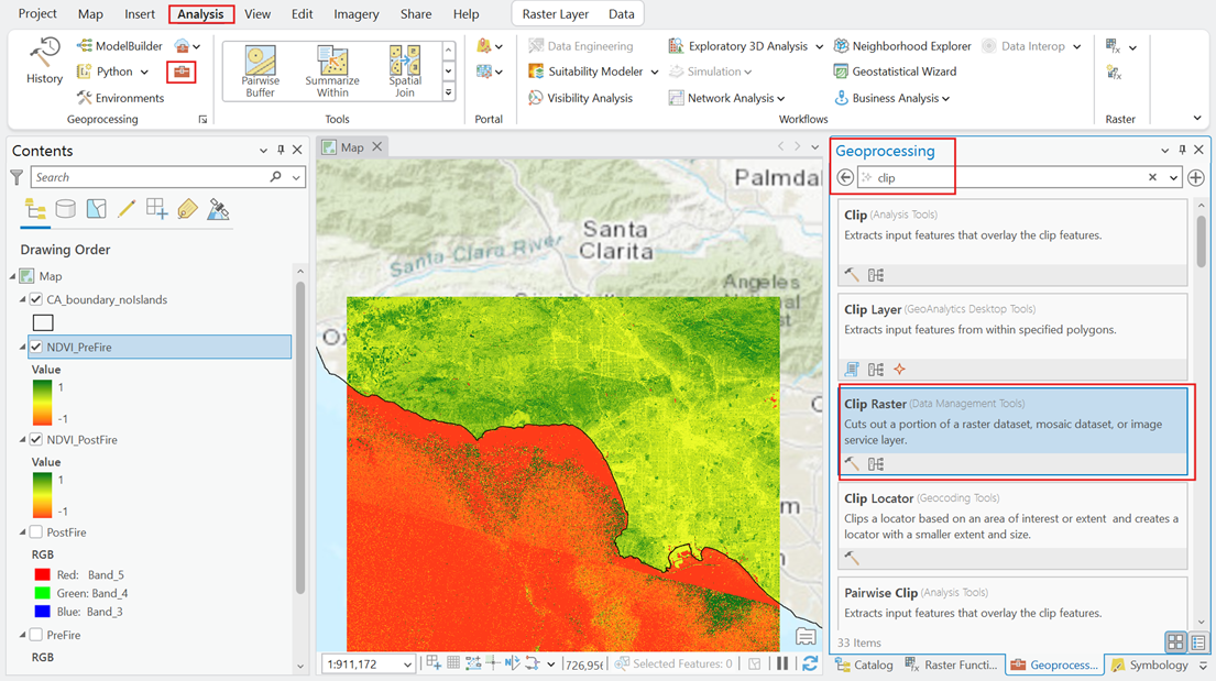
    1. Navigate to the “Analysis” tab and select the toolbox icon which will open the “Geoprocessing” pane.
    2. Search “Clip” and select the “Clip Raster (Data Management Tools).”
      1. Put one of the rasters for the “Input Raster” and the California boundary as “Output Extent.”
      2. Change “Output Raster Dataset” name as desired.
      3. Check the “Use Input Features for Clipping Geometry” box.
      4. Hit “Run” to clip the raster.
    3. Repeat these steps for the second raster.
Image
Image
  1. The symbology of the clipped rasters may reset. Reference step 2 from the previous section—“Apply an NDVI Raster Function”—to reapply symbology.
Image

Calculate Change Detection

Now we will detect changes between the two rasters by subtracting them to quantify differences in pixel values. The resulting raster highlights the degree of change, helping identify areas of vegetation loss or gain. Negative values indicate vegetation loss, while positive values indicate vegetation recovery or regrowth.

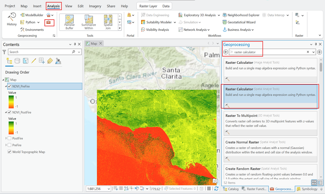
  1. Navigate to the “Analysis” tab and select the toolbox icon which will open the “Geoprocessing” pane.
  2. Search for “Raster Calculator” and select “Raster Calculator (Spatial Analyst Tools).”
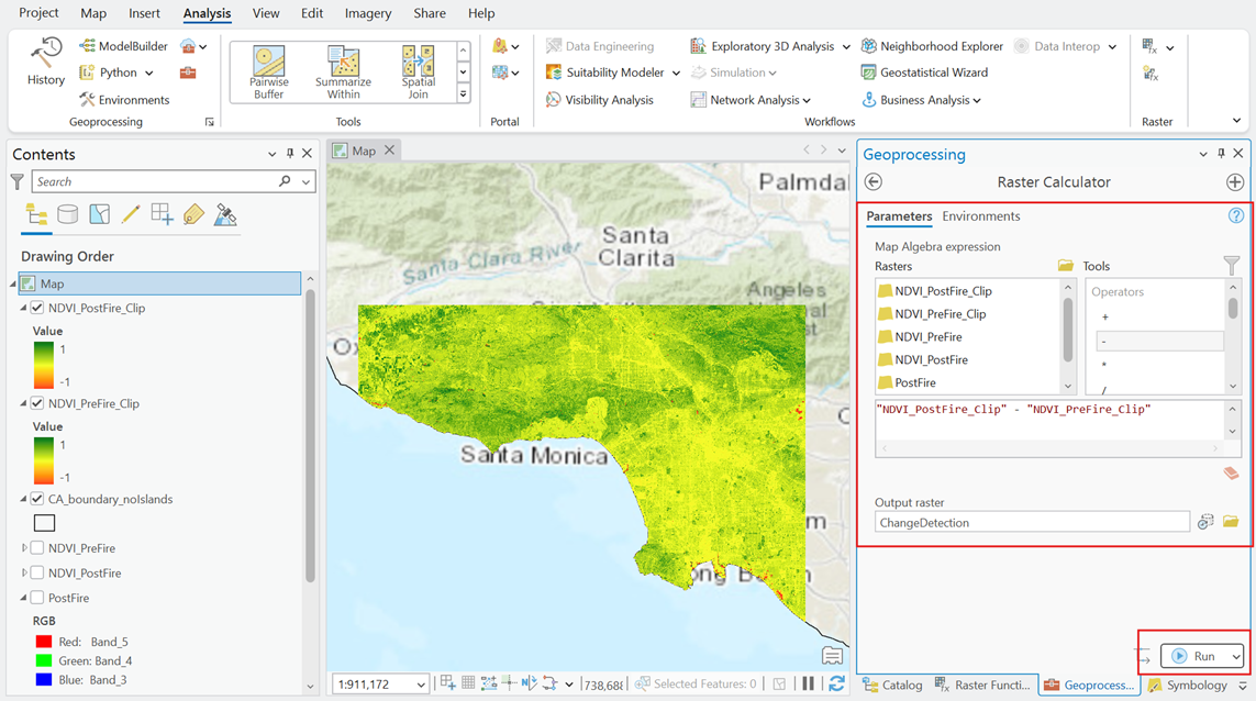
  3. Create the raster calculator map algebra expression by selecting your clipped rasters and the appropriate operator tool.
    1. Select your post fire-clip.
    2. Select the “-“ operator.
    3. Select your pre-fire clip.
    4. Your resulting expression should result in the following format: “NDVI_PostFire_Clip”-“NDVI_PreFireClip.”
  4. Hit “Run.”
Image
Image
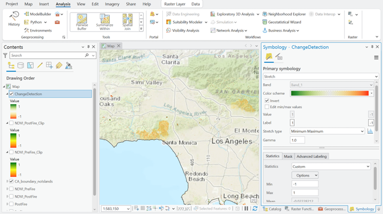
  1. The resulting change detection raster may need its symbology configured for proper and effective visualization.
    1. Open the symbology pane for the change detection layer and adjust as desired.
      1. Set “Statistics” to “Custom” and define “Min” as “-1” and “Max” as “1” to set the proper range.
      2. Change the color scheme to a red-yellow-green color ramp. Check the Invert box to reverse the scheme as needed. We have edited the color ramp for yellow to be “No color” by selecting the color scheme and editing the “Color scheme properties...”

        With this ramp, green will indicate gain in NDVI pixel values, no color will indicate no change in pixel values, and red will indicate loss in NDVI pixel values.

      3. Change the “Stretch type” to “Maximum Minimum.”
      4. Reference ArcGIS Imagery Symbology Documentation to continue to configure the symbology as desired.
Image
  1. Now that we have a change detection layer, you can overlay it with other layers to explore and visualize the extent of vegetation loss and fire impact across the region.
Image

HLS is funded by NASA and is a deliverable of the Satellite Needs Working Group (SNWG), an interagency effort of the U.S. Government dedicated to identifying and addressing Earth observation needs across U.S. civilian federal agencies.

Details

Last Updated

Sept. 23, 2026

Published

Sept. 23, 2026