Workflow Outline

This workflow demonstrates how to use the Common Metadata Repository SpatioTemporal Asset Catalog (CMR STAC) for searching and filtering data; how to use ArcGIS Cloud Storage (ACS) files to enable authenticated access; and how to use ArcGIS configurations (Raster Type and Raster Function Templates) to properly visualize and interact with Harmonized Landsat and Sentinel-2 (HLS) imagery.

Data Used

Tools/Tech Used

  • Earthdata Common Metadata Repository
  • ArcGIS Pro version ≥3.5.2 (requires Esri license)
  • GitHub

Preparing Your Environment with the dkwright Repository

The dkwright arcgis-nasa-earthdata GitHub repository is a supplemental resource that streamlines use of NASA Earthdata in ArcGIS. It provides tools and configurations such as ACS file generation, custom raster types, and raster function templates that enable authenticated access, standardized data handling, and efficient visualization of HLS imagery. ACS files will be used in the STAC Exercise. Parameters (Raster Type and Raster Function Templates) will be used in the STAC Exercise.

Notebooks

The repository contains two notebooks: NASA_Earthdata_ACS_Creator_Web.ipynb and NASA_Earthdata_ACS_Creator_Amazon.ipynb.

We will be using the web version that creates an ACS using a web service provider. This allows ArcGIS Pro to access NASA Earthdata through a standard internet connection using your Earthdata Login. It is best for exploring data, visualizing results, and running smaller analyses directly from your local machine.

The Amazon version creates an ACS connection using the Amazon (S3) service provider, which connects directly to the data stored in Amazon Web Services (AWS). This is ideal for working with large datasets or running analysis at large scale; however, it requires an ArcGIS Pro instance to be running on virtual machine installed from an AWS us-west-2 (Oregon) server.

Follow the steps below to enable these notebooks in your ArcGIS environment:

  1. Download the notebook.
  2. Open ArcGIS Pro. (Optionally, you may also use any other environment with ArcPy installed. For example, JupyterLab.)
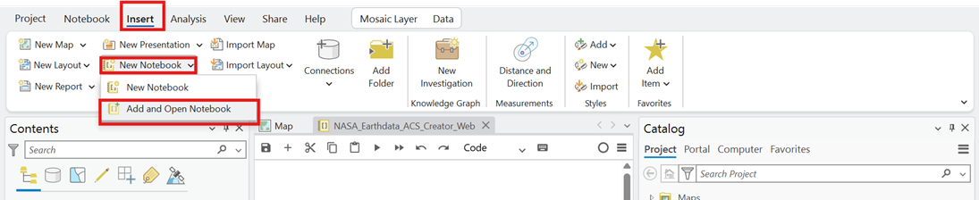
  3. Add the notebook.
    1. Click on the “Insert” tab.
    2. Select “New Notebook.”
    3. “Add and Open Notebook.”
  4. Follow the instructions in NASA_Earthdata_ACS_Creator_Web.ipynb and run the notebook and create ACS connection files.
Image

Parameters

The parameters page contains RasterFunctionTemplates (RFTs) and Raster Type. These control how HLS data is interpreted and visualized in ArcGIS.

Raster Type defines how the imagery is read and structured by ArcGIS, including band order, naming, and metadata handling. It ensures that HLSL (Landsat) and HLSS (Sentinel-2) data are interpreted consistently.

Raster Function Template (RFT) defines how the data is rendered and analyzed, enabling visualizations such as band combinations, indices, dynamic range adjustments, and cloud masking.

  • Download Raster Type files
  • Download RFT files of interest

Finding CMR STAC Endpoint

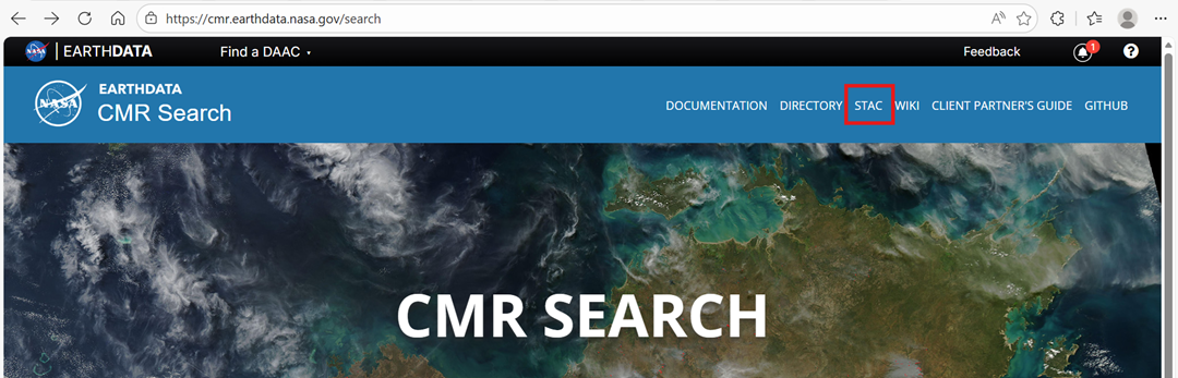
  1. Go to CMR Search and click on “STAC.”
Image
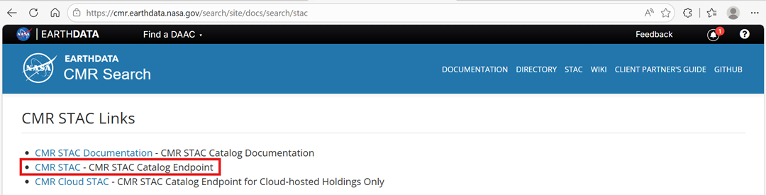
  1. Click on “CMR STAC” to navigate to the CMR STAC Catalog Endpoints.
Image
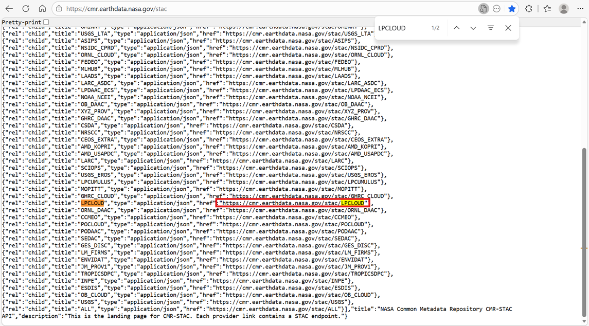
  1. Find the “LPCLOUD” STAC endpoint and record it.
Image

Establishing STAC in ArcGISPro

  1. Open a new project in ArcGISPro.
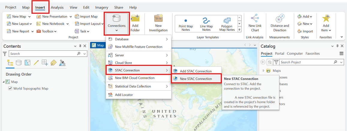
  2. Create a new STAC Connection by following the below menu options:
    1. Insert
    2. Connections
    3. STAC Connection
    4. New STAC Connection
Image
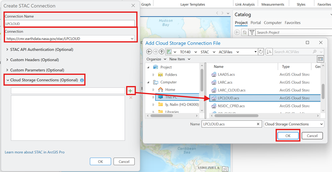
  1. Enter STAC Information:
    1. Enter the “Connection Name” as “LPCLOUD.”
    2. Copy and paste the LPCLOUD CMR STAC endpoint recorded earlier (https://cmr.earthdata.nasa.gov/stac/LPCLOUD).
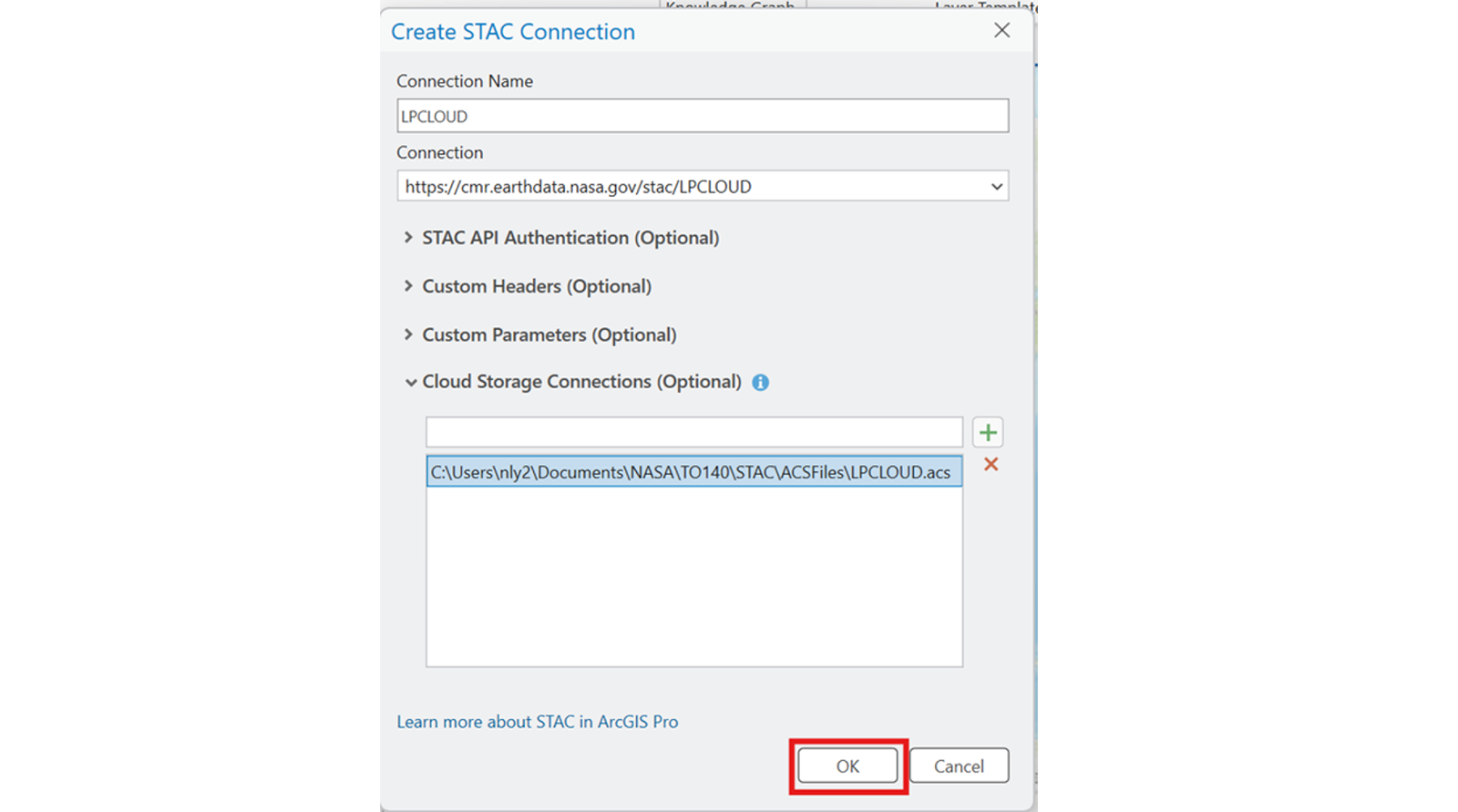
    3. Attach the LPCLOUD.acs file created in the previous activity as a Cloud Storage Connection and click “OK.”
  2. Verify this information and establish connection by clicking “OK.”
Image
Image

Explore STAC Catalog

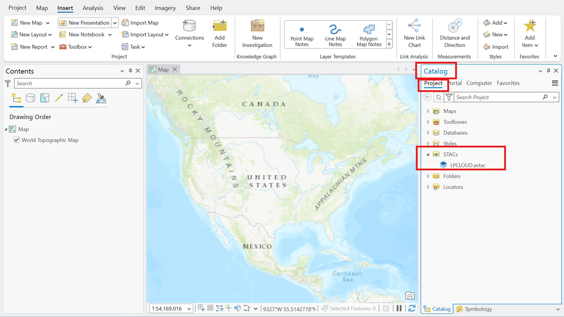
  1. You should now have a STAC folder in your Catalog pane under Project.
    1. Expand the STAC folder.
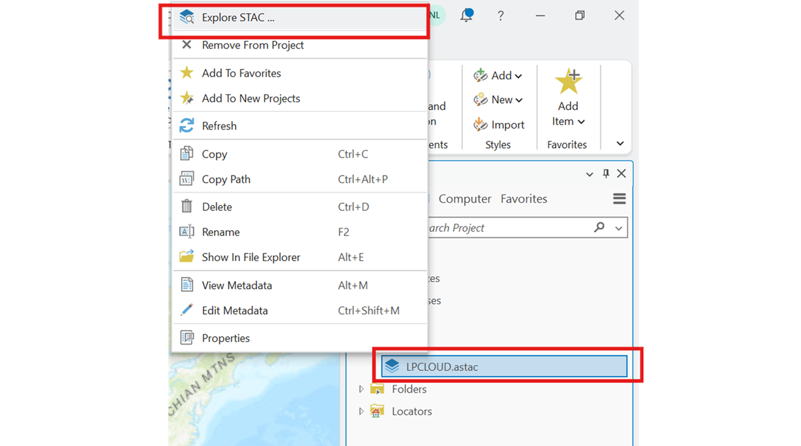
    2. Right click on “LPCLOUD.astac” and select “Explore STAC.”
Image
Image
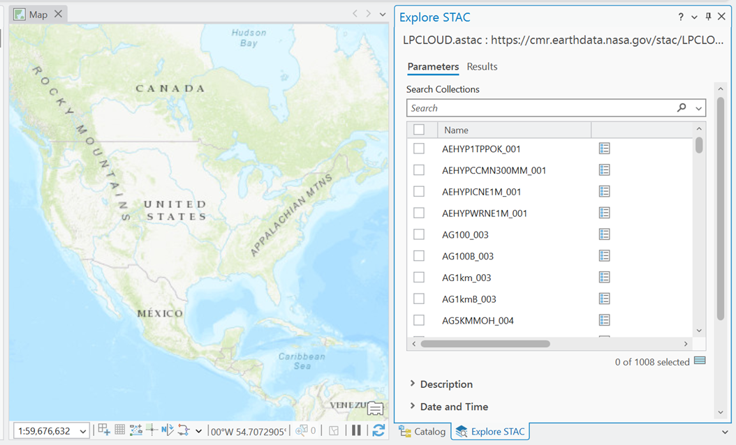
  1. It may take a few moments for all the collections to load before you can explore them. Familiarize yourself with the catalog interface.
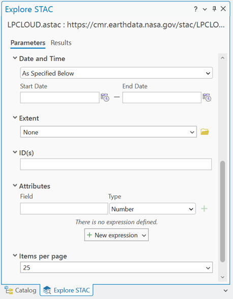
    1. Observe the filter parameters.
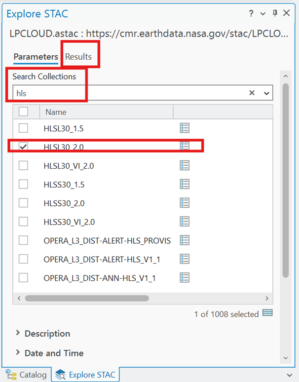
    2. Take this time to explore and change the parameters. Type “hls” into the “Search Collections” bar and then check “HLSL30_2.0”. Click “Results” to see the results of your parameters for the selected collection.
Image
Image
Image
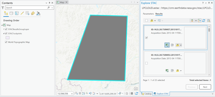
  1. The “Results” interface will allow you to scroll the results. “Next” and “Previous” will allow you to move through the collection catalog. The button selected below will allow you to view the granule footprint. The button to the right will allow you to view the granule properties. The button on the most right will allow you to add the granule to the map or other areas.

    The granule will be displayed in grayscale by default. We will go over how to change band combinations or apply an RFT to properly visualize the data in the next section.
Image

Creating a Mosaic Dataset Example

We will now demonstrate a STAC-enabled workflow by creating a mosaic dataset. We will start by creating an empty mosaic dataset that will hold our data.

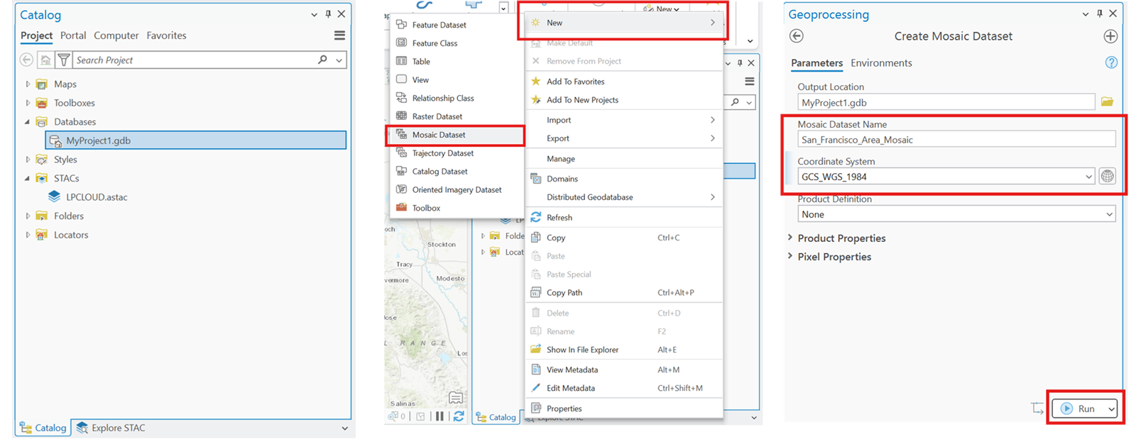
  1. In the catalog pane, navigate to “Databases” and right click on your project’s gdb.
  2. Click “New” and then select “Mosaic Dataset.”
  3. Give the mosaic dataset a name and change the Coordinate System to GCS_WGS_1984 (WGS 1984).
  4. Hit “Run.” Once successfully complete, you should have an empty mosaic dataset in your Contents pane.
Image
  1. We will now add granules to our mosaic dataset. Navigate back to the “Explore STAC” catalog and clear all parameter filters and searches from your exploration.
    1. Type “hls” into the “Search Collections” bar and then check “HLSL30_2.0.”
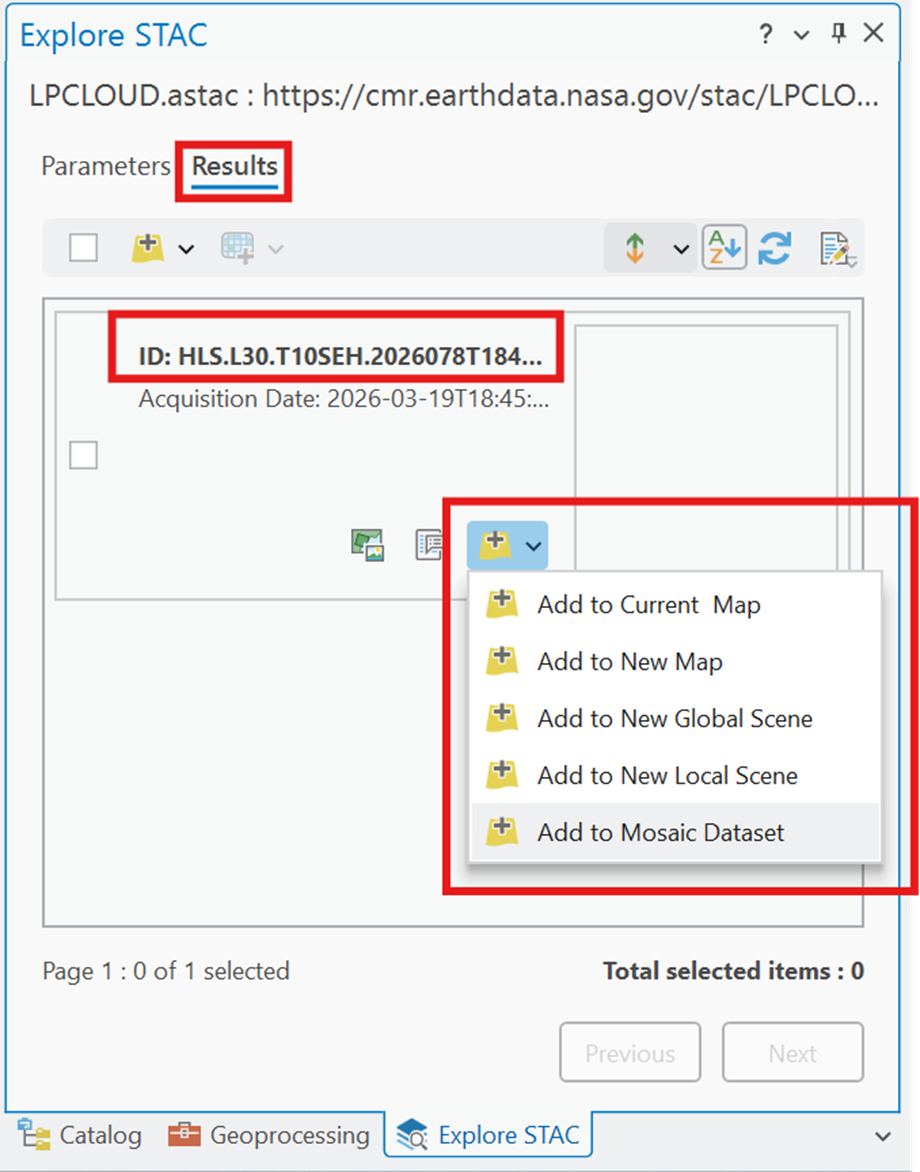
    2. Scroll down to the “ID(s)” parameter and enter in this specific granule: “HLS.L30.T10SEH.2026078T184527.v2.0.”
    3. Hit “Results”. There should be one result. Verify the name. Click “Add to Mosaic Dataset.”
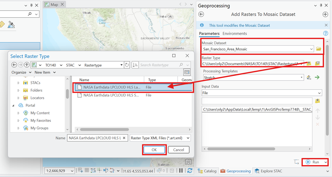
  2. The Geoprocessing Pane should pop up to “Add Rasters to Mosaic Dataset.” For “Mosaic Dataset,” enter in the dataset we created in the previous step.
    1. Change the “Raster Type” to the HLS Landsat Raster Type we downloaded from the dkwright repository.
    2. Hit “OK” to attach the raster type and then hit “Run.”
  3. Repeat this process to add the second granule: “HLS.L30.T10SEG.2026078T184551.v2.0.”
Image
Image
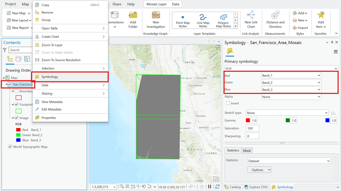
  1. The dataset is displayed in grayscale by default. We can manually change band combinations in the symbology to visualize different composites. We can further configure the imagery with other settings such as Stretch type, Gamma, Saturation, etc. For more information, review ArcGIS Imagery Symbology Documentation.
    1. Right click on the mosaic dataset and open “Symbology.”
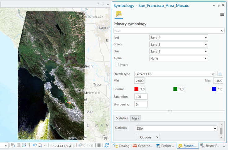
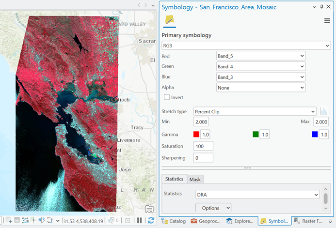
    2. Change band combinations to desired composite. Reference HLS Spectral Bands as needed.

In the screenshots provided below, we can see a true color and false color composite band combinations. The stretch type has been set to Percent Clip and Statistics were set to DRA.

Image
Image
Image
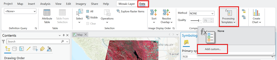
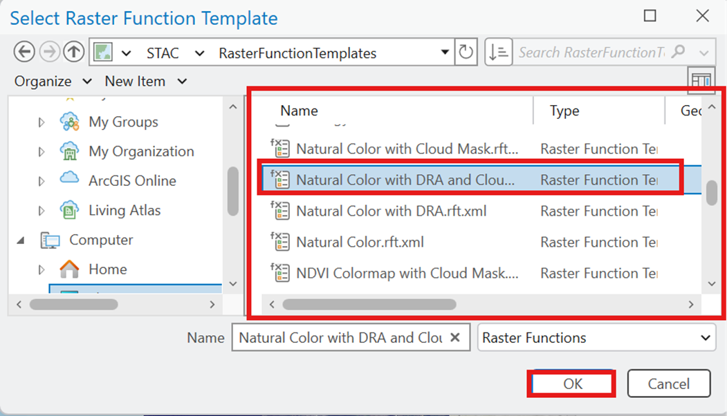
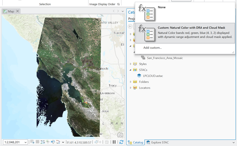
  1. Manual configuration of symbology is a flexible way to customize visuals. However, it can be time-consuming for quick visualizations. We will demonstrate how to apply RFTs to the dataset to automatically render the imagery using predefined symbology.
    1. Navigate to the “Data” tab.
    2. Click “Processing Templates” and then “Add custom…”
    3. Navigate to your downloaded RFTs and select one.
    4. Press “OK” to apply the RFT.
Image
Image
Image

HLS is funded by NASA and is a deliverable of the Satellite Needs Working Group (SNWG), an interagency effort of the U.S. Government dedicated to identifying and addressing Earth observation needs across U.S. civilian federal agencies.

Details

Last Updated

Sept. 23, 2026

Published

Sept. 23, 2026